The English Profile (EP) Visualiser is an example of interpretable interactive machine learning.
The EP Visualiser is a visual user interface which supports exploratory search over a set of approximately 1,200 publically-available FCE texts (Yannakoudakis et al., 2011) using automatically determined discriminative features.
In particular, Briscoe et al. (2010) have used supervised discriminative machine learning techniques to automatically train a linear binary classifier that discriminates passing from failing FCE scripts (CEFR level B2). This model exploits textual features in order to predict whether a script can be classified as passing or failing. A high accuracy on this task was obtained using as features word and part-of-speech (POS) ngrams, among other feature types.
The EP-visualiser aims at supporting their linguistic analysis and interpretation by visualising them, displaying relations with errors as well as other meta-data about the learners, and automatically retrieving scripts instantiating them.
For further details see Yannakoudakis et al., 2012
Feature selection
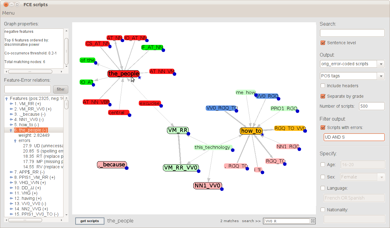
Fig. 1: Front-end of the EP visualiser.
Figure 1 shows the front-end of the user interface (hereafter UI). The Graph → Load data… option on the top left corner of the UI activates the panel (see Figure 2) that enables you to select the features to be displayed. The interface supports the investigation of the top 4,000 highly ranked discriminative features. Features can be displayed according to their association with either passing or failing the exam (positive and negative features respectively), discriminative power, degree (i.e., how many times a feature occurs in the same sentence with other features) and frequency (i.e., in how many sentences a feature occurs). By selecting one of the three radio buttons discriminative power, degree and frequency, the system ranks the features by their discriminative power, degree or frequency respectively (the feature statistics are precomputed using a larger set of FCE scripts) and displays the top N. By filling in the text fields, you can also investigate features whose properties abide to specific ranges of values; for example, features that have a degree of at least 500 or a discriminative power between 200 and 300 (the higher the number, the lower the discriminative power; for example, a discriminative power of 200 means that the feature is ranked as number 200 in the list of discriminative features). Combination of different criteria is also allowed. You can choose to display, for example, the top N features that have a frequency of at least 5,000 and a degree of at least 100, ranked by their discriminative power. Additionally, you can choose to investigate positive or negative features only.
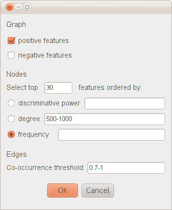
Fig. 2: Selection criteria for dynamic feature-graph building.
The Co-occurrence threshold, located at the bottom of Figure 2, allows you to investigate feature relations. A feature fi is related to a feature fj, if their relative co-occurrence score is within a user-defined range. Feature relations are computed at the sentence level by calculating the proportion of sentences containing a feature fi that also contain a feature fj (given this, the range of values for the Co-occurrence threshold is between 0 and 1). For example, a threshold value of ‘0.9-1’ will group together features that have a high relative co-occurrence score. As shown in Figure 2, when the text fields are filled in, both a minimum a maximum value has to be specified. By hovering the mouse over the text fields, a tooltip text is displayed that shows the range of values you can choose from.
Features are displayed in the central panel where light shades of green and red are used to indicate their association with either passing or failing scripts. Feature relations are shown via highlighting of features when the user hovers the cursor over them, while darker shades of green and red are used to retain the pass/fail information. A field at the bottom right (Search >>) allows searching for features that start with specified characters and highlighting them in blue.
As mentioned in the previous section, you can choose to investigate the top N features that abide to specific selection criteria. However, the top N features might relate to other features from the list of 4,000 (which are not displayed since they are not found in the top N list of features). Blue aggregation markers in the shape of a circle, located at the bottom right of each node, are used to visually display this information. When a node with an aggregation marker is selected (Shift+Left mouse click), the system automatically expands the graph and displays the related features. Now if you wish to return to the original state of the graph, you can select the same node using Shift+Right mouse click.
The Feature–Error relations component on the left of Figure 1 displays a list of the features, ranked by their discriminative power, together with statistics on relations with errors. Feature–error co-occurrences are precomputed at the sentence level by counting out of the number of sentences that contain a feature, the number of sentences that contain a specific error. You can retrieve specific feature–error relations for investigation by filling in the search box above; for example, typing ‘VM_RR ,_because’ (white-space separated) will update the list to display only these two features (and their error relations), while typing ‘*’ will re-display the full list.
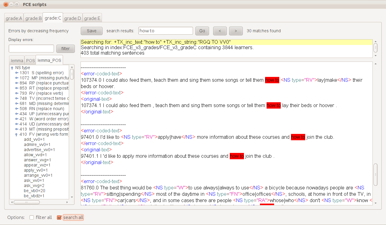
Fig. 3: Sentences, split by grade, containing occurrences of how_to and RGQ_TO_VV0. The list on the left gives error frequencies for matching scripts, including the frequencies of lemmata and POS tags inside an error.
Figure 3 shows the display of the system when the feature bigrams how_to and RGQ_TO_VV0 (see CLAWS2 tagset) are selected. The text area in the centre displays sentences instantiating these features while various colours have been used to differentiate error annotation and XML tags. A search box at the top allows ease of navigation, highlighting keywords in red, while a small text area underneath displays the current search query, the size of the database and the number of matching scripts or sentences. The Errors by decreasing frequency pane on the left shows a list of the errors found in the matching data, ordered by decreasing frequency. Three different tabs (lemma, POS and lemma_POS) provide information about counts of lemmata and POS tags inside an error tag. You can select specific errors for investigation by filling in the search box above; for example, typing ‘RV, RP’ (comma separated) will update the list to display only these two errors, while typing ‘*’ will re-display the full list.
Research on Second Language Acquisition (SLA) highlights the possible effect of a native language (L1) on the learning process. Using the Graph → Select L1 option on the top left corner of Figure 1, you can select the language of interest while the system displays a new window with an identical front-end and functionality. Feature–error statistics are now displayed per L1, while selecting multiple features and clicking on the button get scripts returns scripts written by learners speaking the chosen L1. Although you can already access L1-specific scripts by completing the Languagefield of the right panel in Figure 1, you cannot use this option to perform a sentence-level search which includes meta-data. The Language field, however, is kept since it allows, by means of Boolean queries, simultaneous retrieval of scripts with different L1s, which can be useful for investigating languages belonging to the same family; for example, you can type ‘fr OR es’ (ISO 639-1 language codes) for retrieving scripts written by either French-speaking or Spanish-speaking learners of English.
Briscoe, E.J., B. Medlock & O. Andersen (2010). ‘Automated Assessment of ESOL Free Text Examinations’.
Briscoe, E.J., J. Carroll & R. Watson (2006). ‘The Second Release of the RASP System’. ACL-Coling’06 Interactive Presentation Session, 77–80.
Yannakoudakis, H., E.J. Briscoe & B. Medlock (2011). ‘A new dataset and method for automatically grading ESOL texts’. Proceedings of the 49th Annual Meeting of the Association for Computational Linguistics: Human Language Technologies, Association for Computational Linguistics, 180–189.
Yannakoudakis, H., Briscoe, E.J. & Alexopoulou, T. (2012). Automating Second Language Acquisition Research: Integrating Information Visualisation and Machine Learning. In Proceedings of EACL, Joint Workshop of LINGVIS and UNCLH, Avignon, France.